Pages

Tuesday, March 24, 2020

Delete option in Excel 2010


Hello everyone.

This post I'm going to write about the "Delete" option of Excel 2010.


There are some option to delete the data with this option. Let's learn one by one.
The first option of this "Delete" button is "Delete Cells" option. When you select that option a message box will be seen as below.
Here I'm going to delete the selected cell's data with the given options of the "Delete" window.
When we select the first option named "Shift cells left" of the "Delete" window and click on "Ok" button, the selected cell data will be deleted and the other data of that row will be shifted to left. 
Please refer to the below image to understand this delete option.


The second option is "Shift cell up". When we use this option the result will be, the selected data deleted and the column data of the selected column gone up to the selected cell.

The next two option of the "Delete" window is the same as to the second and the third option of the "Delete" button.

Now let's see the second option of "Delete" button named "Delete Sheet Rows". When we use this option, the entire row which in including the selected cell, will be deleted. 

Action
The Result


Here you can see the "Row 2" has deleted. In this way, you can delete more than one row by selecting any cell counts.
The third option of the "Delete" button is "Delete Sheet Columns". In this way, you can delete one or more columns by selecting cell or cells you want. Here I have selected two cells from the column "M" and column "N". 

The Action
The Result

You can see the column "M" and column "N" have deleted. 

The last option of the "Delete" button is "Delete Sheet". By this option, you can delete the entire Excel sheet. You just need to select a cell on the sheet which you need to delete and click on the "Delete Sheet" option. 
(Click on the image for original size)

Here I have selected "Sheet1" to delete and after click on the "Delete Sheet" option the result will be as below and click on the "Delete" button in the warning message box. Then the sheet1 will be deleted.
(Click on the image for original size)

(Click on the image for original size)
You can use this option to delete data in Excel in different ways. Try this yourself. Thank you.

Alignment of the text in Excel 2010.

Hello everyone,

Today I'm going to write about the alignments of text in Excell 2020. To explain this I will use the below ribbon functions.

Here I have used a cell with a large text ("Text") to show the changes of text with the effect of the above function. 
Among these six options, the first three options are used to change the text alignment by vertically.
Let's try those options first.


And the next three options are used to change the text alignment by horizontally. Please refer to the below image.


Using these options, you can change the text alignment by horizontally and vertically. You can also refer to the  Change the orientation of a text post to learn how to change the orientation of a text in Excel 2020.  Thank you.

Monday, March 23, 2020

Customize the Ribbon in Excel 2010 - Part 05 ( Reset , Export/Import the ribbon data)

Hello,

Today post I'm going to write how to Export/Import the ribbon data in Excel 2020. 
Assume that you need to keep your ribbon changes as a backup before we reset the ribbon. Then you can be used this option.

Let's add some new tabs and tab groups to check this option. We have already learnt how to add tabs and tab groups to the ribbon. If you have missed those posts, please visit and read from below links.

01) Customize the Ribbon in Excel 2020 - Part 01
02) Customize the Ribbon in Excel 2020 - Part 02

Ok. Refer to the below image and I have added some new tabs and tab groups to the ribbon.


Now let's see how to export the ribbon data.
You just go to the "Import/Export" button. Then you will be seen yow options relevant to the "Export/Import" button as below image.


In here we have to use the second option named "Export all customization". Click on that option and you will be seen "Save File" window as below and you need to give a name or keep the automated name to be saved the exporting file. And also select a location to save the file.


The file will be saved as a ".exportedUI" file. Do not change the extension for any reason. 
Now click on the "Save" button and check the saved file in the given location.

This is the saved file of my export.
Then you can reset your ribbon and after you can import this file to re-arrange your customization to the Excel ribbon when you need. After you reset the ribbon data, the tab list will be appeared as below and you can see there are only inbuilt tabs available.

Ok. Let's check the Import option.
Click on the "Export/Import" button and click on the "Import customization file"option. Then you will appear "File Open" window and need to find the exported file from the saved location and just click on the "Open" button.

After you click on the "Open" button, a message box will appear as below.


Click on the "Yes" button and check the tab list. Now you can see the exported data have restored to the tab list.


Alright. This is about export and imports the ribbon and Quick Access Toolbar data inExcel 2020. Try these yourself and check all actions out what we have learnt. Thank you.

Sunday, March 22, 2020

Customize the Ribbon in Excel 2010 - Part 04 ( Reset , Export/Import the ribbon data)

Hello everyone,

In today post I'm going to write how to reset and export or import the ribbon data.
We have to use the Excel Options window to do this function also. Go to the "Excel Options" window and select the "Customize Ribbon" option.
Please see the below image and we need to use the red colour highlighted area to execute the above functions.


See the below image to find the inbuilt tab details.


These tabs will not be changed when we reset the tab data. Let's see how will the "Reset" option work.
We have already learnt how to add new tabs to the ribbon. To execute the reset option we need to add new tabs or new groups by changing the inbuilt data of the ribbon. Refer to the below image.


Ok. Now we just click on the reset button and see what will the result.

When we click on the "Reset" button, it will appear two options to yous how we need to reset the ribbon data. In the "Reset only selected Ribbon tab" option, we can choose some inbuilt tabs not to change their data.
And the "Reset all customizations" option, we can bring the ribbon to the inbuilt situation. It means this option will clear all the customization which you have done. Please refer to the below images.


Click on the "Reset all customization" option and then a message box will be appeared as below.

In this reset option the "Quick Access Toolbar" also be reset to the inbuilt situation.
After we click the "Yes" button the ribbon details will be changed as billow. Here you can see the ribbons which we have created are not there anymore.


Ok. The next option we have to learn is the "Import/Export" option.
Assume that you need to keep your ribbon changes as a backup before we reset the ribbon. Then you can be used this option. I will write about this option in the next post. Till then try this out yourself.

Customize the Ribbon in Excel 2010 - Part 03

Hello everyone,

This is part 03 of "Customize the Ribbon in Excel 2020". In this post, I'm going to write about how to change the positions of tabs and tabs data in the ribbon. to do this wee need to open the "Excel Options" window.

  •  File → Options
  • Excel Options → Customize Ribbon
Then, you need to select the tab which you need to move up or down.
In here I have selected "My Tab" to move. After selecting a tab, just go to the red colour highlighted button (Up button) and click on that. 


the result will be as below.

In this way, you can change the tab groups and group options' positions also. After changing the positions, the ribbon will appear as bellow and the changes have done.


This is the way to change the position of the tabs, tab groups and options of those groups. 

Customize the Ribbon in Excel 2010 - Part 02

Welcome to the "Customize the Ribbon in Excel 2020 - Part 02".

We have already created a tab named "My Tab" in the ribbon and now we going to add "Groups" to the "My Tab"
To do this you need to click on the "+" mark of "My Tab". Then The "My Tab" will extend and show like below image.


When we create a new tab, It is included a group named "New Group(Custom)". We can rename this group with a name which you need. Just select an icon and enter a name to your group and click on the "Ok" button.


Then the new group will be renamed and appeared the tab achieve like below.

And then we need to add buttons/options to the "My Group". To do this, you just need to select the "My Group" and go to the left side and select on an option which you need to add to your group and then click on the "Add" button. Then the selected option will be added to your group.


In this way, you can add more options to your group(My Group). After you add some options, the "My Tab" will appear as bellow.

After selecting the options just click on the "Ok" button and check your ribbon. The ribbon will appear as bellow.


In this way, you can customize and design a tan to the Excel ribbon.  
And also we can change the positions of this tab, the tab group and the group options' as well. I will write about that in the next post. Till then try this out. Thank you.

Saturday, March 21, 2020

Customize the Ribbon in Excel 2010 - Part 01

Hi everyone,

Today I'm going to write how to customize the Ribbon in Excell 2020.
There are lots of inbuilt options on the ribbon in Excel. If we need to add our own group to the ribbon, there is an option to customize the ribbon and to insert our own group into the ribbon.

First, you need to go to a free space of the ribbon and right-click on that space. Then you will appear as below.

After you need to click on the "Customize the Ribbon" option. Then bellow window will appear.


This window is the Excel Options window. You can be also found this window from below path.

  • File → Options.
After you open this window you will be seen all the currently available tabs and tab groups are available here. In here you can not add any options to the existing groups. If you try to do that below message will appear.

Hence, If we need to create our own group you need to add a new group. In here I would like to add a tab to ribbon and after will add groups to that ribbon. 
To do this, just right-click on the existing tab and click on the "Add New Tab" option.


The result will be as below.
Then you can rename the new tab with a new name. I will change this as "My Tab"


Now the tab archive will be shown as below with your tab and then click "Ok".


The new ribbon of your Excel will be shown as below. "My Tab" is there.


Ok. After that, we have to add tab groups into this tab. I will write it in the next post. Till then try this out. 

Change the orientation of a text in excel 2010

Hello everyone,

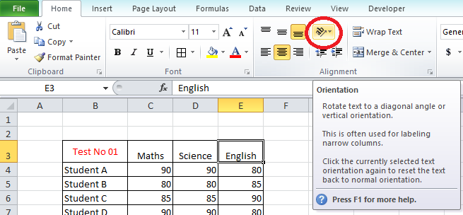
Today I'm going to write how to change the orientation of text in Excel. We can do this with below tow option. See the below image.

Option 01


Option 02

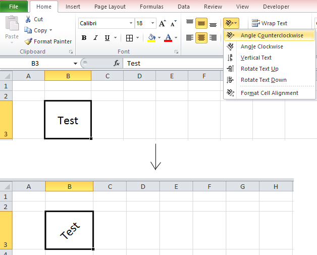
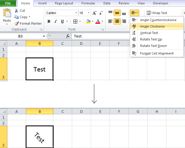
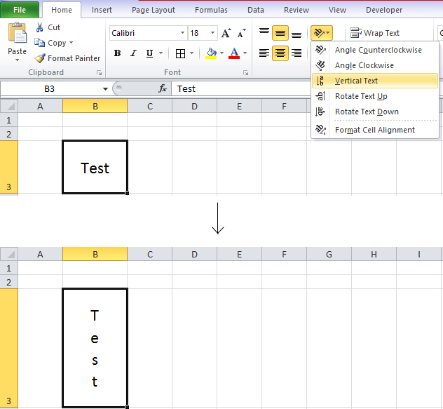
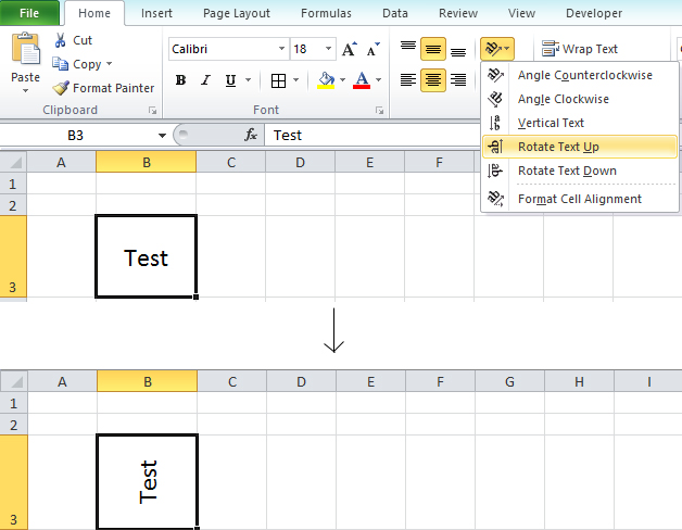
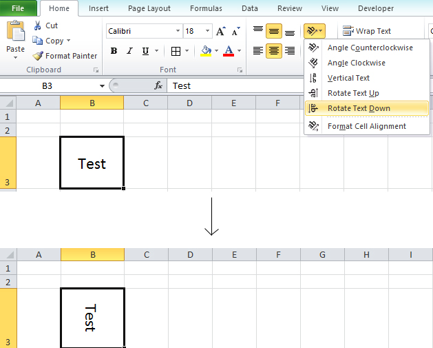
Now let's see how it works. Here I'm using below images to explain the option and result.

01) The Angle Counterclockwise option

02) Angle Clockwise Option
03) Verticle text Option

04) Rotate Text Up option
05) Rotate Text Down Option
And with the 6th option "Format Cell Alignment", we can see more options to change the orientation of a text.
The "Format Cell Alignment" window will be appeared as below. The "Format Cell" window will open with this option and there is an option named "Alignment" to change the orientation of a text.


You can change the orientation of a text by using the red colour highlighted area.